Showcases of tfplot
This guide shows a quick tour of the tfplot library. Please skip the setup section of this document.
[5]:
import tfplot
tfplot.__version__
[5]:
'0.3.0.dev0'
Setup: Utilities and Data
In order to see the images generated from the plot ops, we introduce a simple utility function which takes a Tensor as an input and displays the resulting image after executing it in a TensorFlow session.
You may want to skip this section to have the showcase started.
[6]:
import tensorflow as tf
sess = tf.InteractiveSession()
[7]:
def execute_op_as_image(op):
    """
    Evaluate the given `op` and return the content PNG image as `PIL.Image`.

    - If op is a plot op (e.g. RGBA Tensor) the image or
      a list of images will be returned
    - If op is summary proto (i.e. `op` was a summary op),
      the image content will be extracted from the proto object.
    """
    print ("Executing: " + str(op))
    ret = sess.run(op)
    plt.close()

    if isinstance(ret, np.ndarray):
        if len(ret.shape) == 3:
            # single image
            return Image.fromarray(ret)
        elif len(ret.shape) == 4:
            return [Image.fromarray(r) for r in ret]
        else:
            raise ValueError("Invalid rank : %d" % len(ret.shape))

    elif isinstance(ret, (str, bytes)):
        from io import BytesIO
        s = tf.Summary()
        s.ParseFromString(ret)
        ims = []
        for i in range(len(s.value)):
            png_string = s.value[i].image.encoded_image_string
            im = Image.open(BytesIO(png_string))
            ims.append(im)
        plt.close()
        if len(ims) == 1: return ims[0]
        else: return ims

    else:
        raise TypeError("Unknown type: " + str(ret))
and some data:
[8]:
def fake_attention():
import scipy.ndimage
attention = np.zeros([16, 16], dtype=np.float32)
attention[(11, 8)] = 1.0
attention[(9, 9)] = 1.0
attention = scipy.ndimage.filters.gaussian_filter(attention, sigma=1.5)
return attention
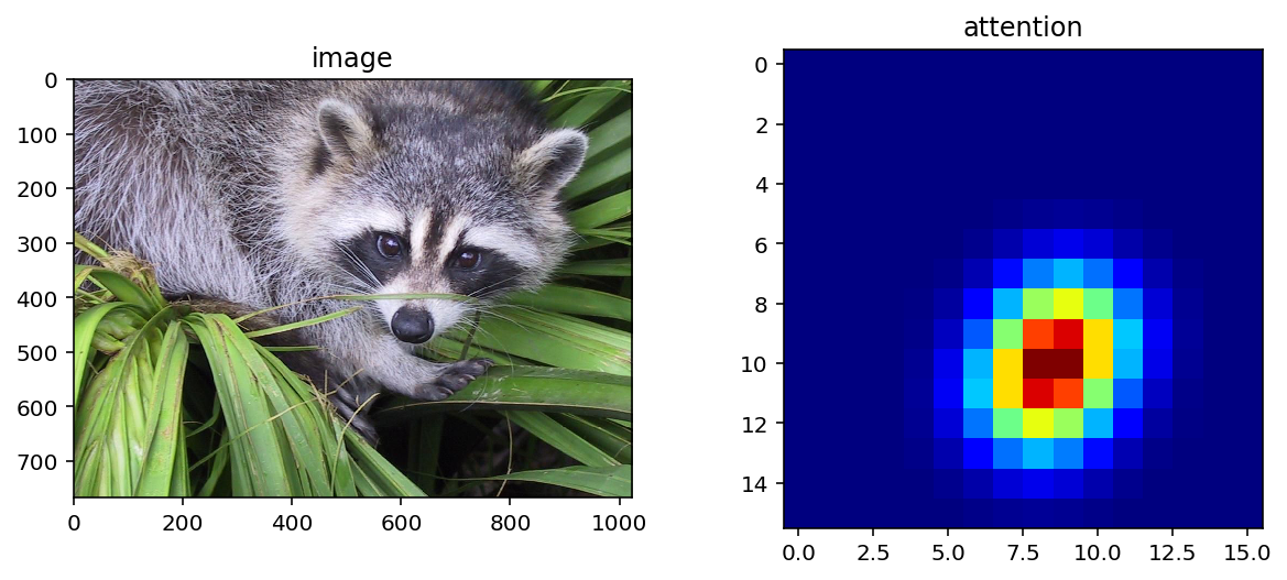
sample_image = scipy.misc.face()
attention_map = fake_attention()
# display the data
fig, axs = plt.subplots(1, 2, figsize=(10, 4))
axs[0].imshow(sample_image); axs[0].set_title('image')
axs[1].imshow(attention_map, cmap='jet'); axs[1].set_title('attention')
plt.show()
And we finally wrap these numpy values into TensorFlow ops:
[9]:
# the input to plot_op
image_tensor = tf.constant(sample_image, name='image')
attention_tensor = tf.constant(attention_map, name='attention')
print(image_tensor)
print(attention_tensor)
Tensor("image:0", shape=(768, 1024, 3), dtype=uint8)
Tensor("attention:0", shape=(16, 16), dtype=float32)
1. tfplot.autowrap: The Main End-User API
Use tfplot.autowrap to design a custom plot function of your own.
Decorator to define a TF op that draws plot
With tfplot.autowrap, you can wrap a python function that returns matplotlib.Figure (or AxesSubPlot) into TensorFlow ops, similar as in tf.py_func.
[10]:
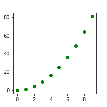
@tfplot.autowrap
def plot_scatter(x, y):
    # NEVER use plt.XXX, or matplotlib.pyplot.
    # Use tfplot.subplots() instead of plt.subplots() to avoid thread-safety issues.
    fig, ax = tfplot.subplots(figsize=(3, 3))
    ax.scatter(x, y, color='green')
    return fig

x = tf.constant(np.arange(10), dtype=tf.float32)
y = tf.constant(np.arange(10) ** 2, dtype=tf.float32)
execute_op_as_image(plot_scatter(x, y))
Executing: Tensor("plot_scatter:0", shape=(?, ?, 4), dtype=uint8)
[10]:
We can create subplots as well. Also, note that additional arguments (i.e. kwargs) other than Tensor arguments (i.e. positional arguments) can be passed.
[11]:
@tfplot.autowrap
def plot_image_and_attention(im, att, cmap=None):
    fig, axes = tfplot.subplots(1, 2, figsize=(7, 4))
    fig.suptitle('Image and Heatmap')
    axes[0].imshow(im)
    axes[1].imshow(att, cmap=cmap)
    return fig

op = plot_image_and_attention(sample_image, attention_map, cmap='jet')
execute_op_as_image(op)
Executing: Tensor("plot_image_and_attention:0", shape=(?, ?, 4), dtype=uint8)
[11]:

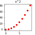
Sometimes, it can be cumbersome to create instances of fig and ax. If you want to have them automatically created and injected, use a keyword argument named fig and/or ax:
[12]:
@tfplot.autowrap(figsize=(2, 2))
def plot_scatter(x, y, *, ax, color='red'):
    ax.set_title('x^2')
    ax.scatter(x, y, color=color)

x = tf.constant(np.arange(10), dtype=tf.float32)
y = tf.constant(np.arange(10) ** 2, dtype=tf.float32)
execute_op_as_image(plot_scatter(x, y))
Executing: Tensor("plot_scatter_1:0", shape=(?, ?, 4), dtype=uint8)
[12]:
2. Wrapping Matplotlib’s AxesPlot or Seaborn Plot
You can use tfplot.autowrap (or raw APIs such as tfplot.plot, etc.) to plot anything by writing a customized plotting function on your own, but sometimes we may want to convert already existing plot functions from common libraries such as matplotlib and seaborn.
To do this, you can still use tfplot.autowrap.
Matplotlib
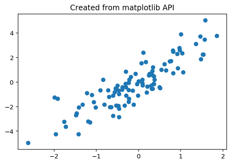
Matplotlib provides a variety of plot methods defined in the class AxesPlot (usually, ax).
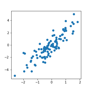
[13]:
rs = np.random.RandomState(42)
x = rs.randn(100)
y = 2 * x + rs.randn(100)

fig, ax = plt.subplots()
ax.scatter(x, y)
ax.set_title("Created from matplotlib API")
plt.show()
We can wrap the Axes.scatter() method as TensorFlow op as follows:
[14]:
from matplotlib.axes import Axes
tf_scatter = tfplot.autowrap(Axes.scatter, figsize=(4, 4))

plot_op = tf_scatter(x, y)
execute_op_as_image(plot_op)
Executing: Tensor("scatter:0", shape=(?, ?, 4), dtype=uint8)
[14]:
Seaborn
Seaborn provides many useful axis plot functions that can be used out-of-box. Most of functions for drawing an AxesPlot will have the ax=... parameter.
See seaborn’s example gallery for interesting features seaborn provides.
[15]:
import seaborn as sns

assert sns.__version__ >= '0.8', \
    'Use seaborn >= v0.8.0, otherwise `import seaborn as sns` will affect the default matplotlib style.'
barplot: (Discrete) Probability Distribution
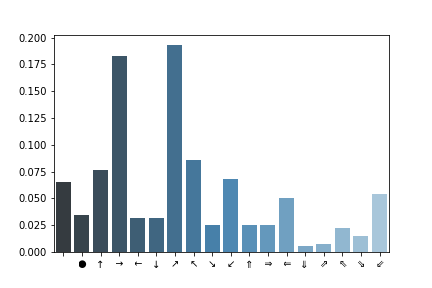
[16]:
# https://seaborn.pydata.org/generated/seaborn.barplot.html

y = np.random.RandomState(42).normal(size=[18])
y = np.exp(y) / np.exp(y).sum() # softmax
y = tf.constant(y, dtype=tf.float32)

ATARI_ACTIONS = [
    '⠀', '●', '↑', '→', '←', '↓', '↗', '↖', '↘', '↙',
    '⇑', '⇒', '⇐', '⇓', '⇗', '⇖', '⇘', '⇙' ]
x = tf.constant(ATARI_ACTIONS)

op = tfplot.autowrap(sns.barplot, palette='Blues_d')(x, y)
execute_op_as_image(op)
Executing: Tensor("barplot:0", shape=(?, ?, 4), dtype=uint8)
[16]:

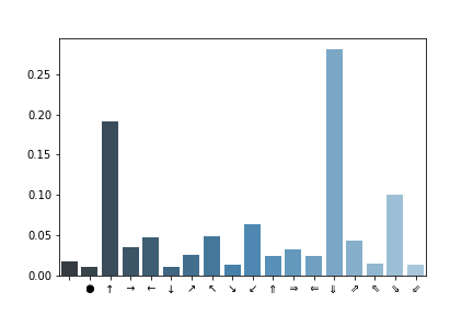
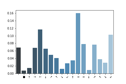
[17]:
y = np.random.RandomState(42).normal(size=[3, 18])
y = np.exp(y) / np.exp(y).sum(axis=1).reshape([-1, 1]) # softmax example-wise
y = tf.constant(y, dtype=tf.float32)

ATARI_ACTIONS = [
    '⠀', '●', '↑', '→', '←', '↓', '↗', '↖', '↘', '↙',
    '⇑', '⇒', '⇐', '⇓', '⇗', '⇖', '⇘', '⇙' ]
x = tf.broadcast_to(tf.constant(ATARI_ACTIONS), y.shape)

op = tfplot.autowrap(sns.barplot, palette='Blues_d', batch=True)(x, y)
for im in execute_op_as_image(op):
    display(im)
Executing: Tensor("barplot_1/PlotImages:0", shape=(3, ?, ?, 4), dtype=uint8)
Heatmap
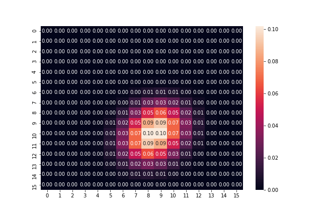
Let’s wrap seaborn’s heatmap function, as TensorFlow operation, with some additional default kwargs. This is very useful for visualization.
[18]:
# @seealso https://seaborn.pydata.org/examples/heatmap_annotation.html
tf_heatmap = tfplot.autowrap(sns.heatmap, figsize=(9, 6))

op = tf_heatmap(attention_map, cbar=True, annot=True, fmt=".2f")
execute_op_as_image(op)
Executing: Tensor("heatmap:0", shape=(?, ?, 4), dtype=uint8)
[18]:
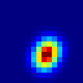
What if we don’t want axes and colorbars, but only the map itself? Compare to plain tf.summary.image, which just gives a grayscale image.
[19]:
# print only heatmap figures other than axis, colorbar, etc.
tf_heatmap = tfplot.autowrap(sns.heatmap, figsize=(4, 4), tight_layout=True,
                             cmap='jet', cbar=False, xticklabels=False, yticklabels=False)

op = tf_heatmap(attention_map, name='HeatmapImage')
execute_op_as_image(op)
Executing: Tensor("HeatmapImage:0", shape=(?, ?, 4), dtype=uint8)
[19]:
And Many More!
This document has covered a basic usage of tfplot, but there are a few more:
tfplot.contrib: contains some off-the-shelf functions for creating plot operations that can be useful in practice, in few lines (without a hassle of writing function body). See [contrib.ipynb] for more tour of available APIs.tfplot.plot(),tfplot.plot_many(), etc.: Low-level APIs.tfplot.summary: One-liner APIs for creating TF summary operations.
[21]:
import tfplot.contrib
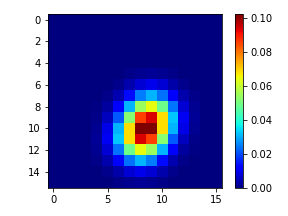
For example, probmap and probmap_simple create an image Tensor that visualizes a probability map:
[22]:
op = tfplot.contrib.probmap(attention_map, figsize=(4, 3))
execute_op_as_image(op)
Executing: Tensor("probmap:0", shape=(?, ?, 4), dtype=uint8)
[22]:
[23]:
op = tfplot.contrib.probmap_simple(attention_map, figsize=(3, 3), vmin=0, vmax=1)
execute_op_as_image(op)
Executing: Tensor("probmap_1:0", shape=(?, ?, 4), dtype=uint8)
[23]:

That’s all! Please take a look at API documentations and more examples if you are interested.